What is the difference between XLOOKUP and VLOOKUP?

XLOOKUP defaults to exact match, can search in any direction, doesn't break when columns are inserted, has a built-in if_not_found argument, and can return multiple columns at once. VLOOKUP defaults to approximate match, only works left-to-right, and relies on a hard-coded column index that breaks if you insert or delete columns.

Is XLOOKUP available in all versions of Excel?

No. XLOOKUP is available in Excel for Microsoft 365, Excel for the web, Excel 2021, and Excel 2024. It is not available in Excel 2019, Excel 2016, or earlier — those versions will show a #NAME? error and require INDEX/MATCH or VLOOKUP instead.

Can XLOOKUP return multiple values?

Yes. If you pass a multi-column range as the return_array (e.g. C2:E8), XLOOKUP will spill all matching columns horizontally into adjacent cells with a single formula.

How to Use XLOOKUP in Excel (Step-by-Step Guide)

XLOOKUP is the modern replacement for VLOOKUP and HLOOKUP in Excel. It is faster to write, more flexible, and avoids the column-index pitfalls that break older lookup formulas. This guide walks you through the syntax, a real worked example with screenshots, and the advanced patterns analysts use every day.

What is XLOOKUP?

XLOOKUP is an Excel function that searches a range for a value and returns a corresponding result from another range. It replaces both VLOOKUP and HLOOKUP with a single, more powerful formula that works in any direction (left, right, up, or down) and defaults to exact match — eliminating one of the most common sources of bugs in financial models.

XLOOKUP is available in Excel for Microsoft 365, Excel for the web, Excel 2021, and Excel 2024. It is not available in older perpetual versions such as Excel 2019 and Excel 2016 — those will show #NAME? and require INDEX/MATCH or VLOOKUP as a fallback.

XLOOKUP Syntax

The full syntax is:

=XLOOKUP(lookup_value, lookup_array, return_array, [if_not_found], [match_mode], [search_mode])

lookup_value — what you are searching for.
lookup_array — the range to search in.
return_array — the range to return a value from.
[if_not_found] — optional value to return if no match (e.g. "N/A").
[match_mode] — 0 = exact (default), -1 = exact or next smaller, 1 = exact or next larger, 2 = wildcard.
[search_mode] — 1 = first to last (default), -1 = last to first.

Step-by-Step XLOOKUP Example

We will look up a company's Revenue by entering its ticker symbol. Below is the dataset: tickers in column B, financial metrics in columns C–E, and a small input panel in columns G–H where the user types a ticker into H1.

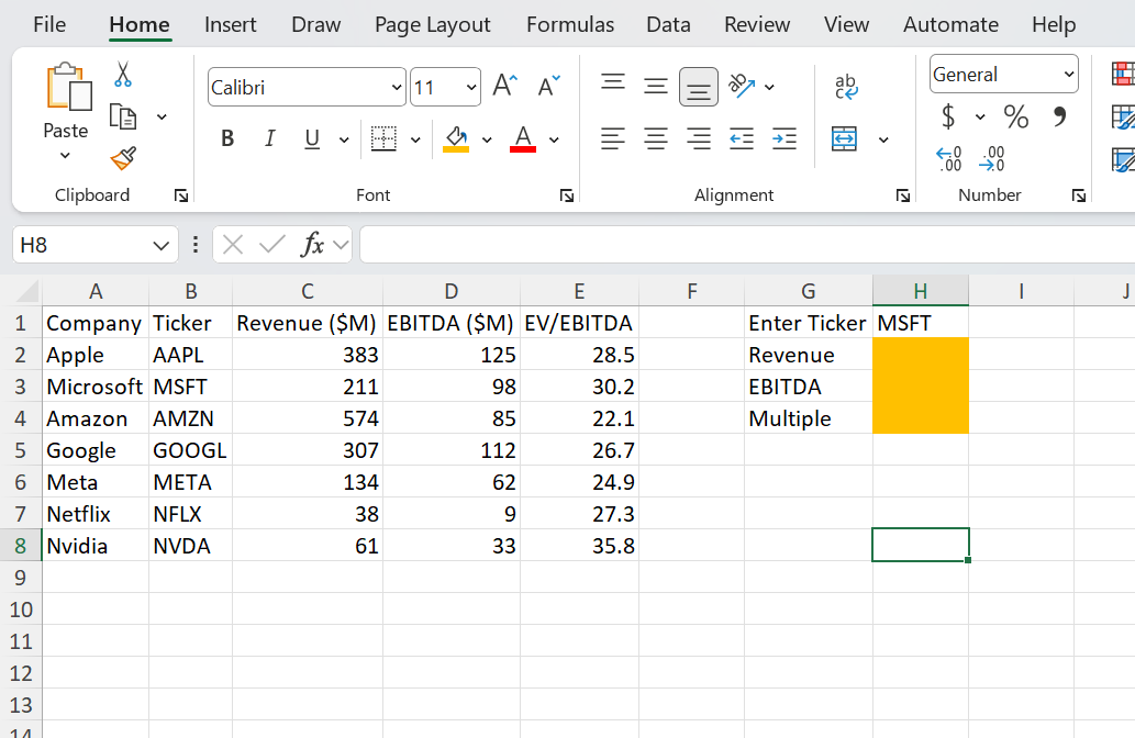
Excel sample dataset showing company tickers in column B with Revenue, EBITDA, and EV/EBITDA in columns C through E, and an input panel in columns G and H — Sample dataset: tickers in column B with financial metrics in columns C–E. The user enters a ticker into H1.

Step 1 — Click the cell where you want the result

Select cell H2 (next to the "Revenue" label).

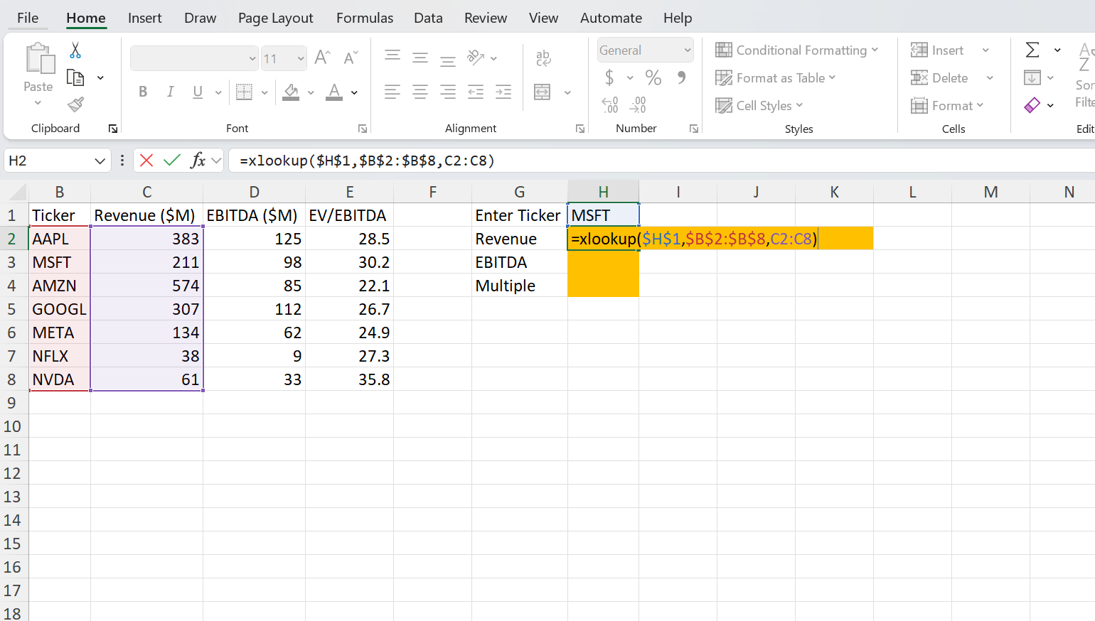
Step 2 — Type the formula

Enter:

=XLOOKUP($H$1, $B$2:$B$8, C2:C8)

The dollar signs lock the lookup cell and lookup array so the formula can be copied down to retrieve EBITDA and EV/EBITDA without breaking.

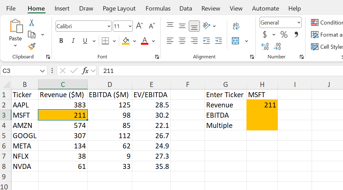
Excel formula bar showing =XLOOKUP($H$1,$B$2:$B$8,C2:C8) being entered into cell H2 with the lookup and return ranges highlighted — The XLOOKUP formula in cell H2 — Excel highlights the lookup array (B2:B8) and the return array (C2:C8).

Step 3 — Press Enter

Excel returns 211 — Microsoft's revenue. Change H1 to any other ticker and the result updates instantly.

Excel result showing 211 returned in cell H2 after looking up MSFT in the ticker column — Result: 211 returned for MSFT Revenue. The matched row in column B is highlighted.

XLOOKUP vs VLOOKUP

Feature	VLOOKUP	XLOOKUP
Default match	Approximate (when match argument is omitted)	Exact (safe default)
Lookup direction	Left-to-right only	Any direction
Column index	Hard-coded number	Reference to actual range
Breaks if columns inserted	Yes	No
Built-in if_not_found	No — typically wrapped in IFERROR or IFNA	Yes (built-in argument)
Returns multiple columns	No	Yes (spills)

Advanced XLOOKUP Examples

Return multiple columns at once

Using the same ticker dataset, you can return Revenue, EBITDA, and EV/EBITDA in a single formula by passing the entire C2:E8 block as the return array:

=XLOOKUP($H$1, $B$2:$B$8, C2:E8)

The result spills three values horizontally — no need to write three separate formulas.

Approximate match (for sorted numeric ranges)

For bands or thresholds — such as tax brackets, credit ratings, or commission tiers — use match_mode = -1 to find the largest value less than or equal to the lookup value. This is not for exact-ID lookups like the ticker example above.

=XLOOKUP(income, bracket_floor, tax_rate, "N/A", -1)

If income is 85,000 and your bracket_floor column is sorted ascending (0, 50000, 100000, 200000), XLOOKUP returns the rate associated with the 50,000 bracket.

Handle missing values gracefully

=XLOOKUP($H$1, $B$2:$B$8, C2:C8, "Not found")

Type a ticker that doesn't exist (e.g. XYZ) and you'll see Not found instead of #N/A.

Common XLOOKUP Mistakes

Forgetting absolute references. If you copy your formula down, lock the lookup cell and lookup array with $ signs.
Mismatched array sizes. The lookup_array and return_array must have the same number of rows (or columns).
Using XLOOKUP in older Excel. XLOOKUP isn't available in Excel 2019, Excel 2016, or earlier perpetual versions. Files using it will show #NAME? when opened there.
Approximate match on unsorted data. match_mode = -1 or 1 requires the lookup array to be sorted.

Pro Tips for Analysts

Pair XLOOKUP with data validation dropdowns to build interactive ticker or scenario selectors in financial models.
Use the spill behavior (returning multiple columns) to keep models lean — one formula instead of three or four.
Combine XLOOKUP with SUMIFS or INDEX for two-dimensional lookups across rows and columns.
Always wrap user-facing lookups with the if_not_found argument to avoid #N/A errors propagating through your model.

Frequently Asked Questions

Related Training

Ready to Get Faster?

Start practicing with hands-on Excel drills designed for financial professionals.