VLOOKUP in Excel: Step-by-Step Guide (With Examples & Formula)
VLOOKUP is one of the most widely used functions in Excel — and one of the most error-prone. This guide walks through the syntax, a real worked example with screenshots, the most common errors (and how to fix them), and when to switch to XLOOKUP. Built for analysts who need lookup formulas that don't break in financial models.
See also: Excel Skill Test — Benchmark your spreadsheet level
What is VLOOKUP?
VLOOKUP ("vertical lookup") searches the first column of a table for a value and returns a corresponding value from another column in the same row. It's widely used in financial modeling, data analysis, and reporting — to pull employee details from an HR table, financials from a comps sheet, or prices from a product catalog.
It has three well-known limitations:
- It only searches left-to-right (the lookup column must be the leftmost).
- It uses a hard-coded column index number, which breaks if you insert or delete columns.
- It defaults to approximate match when the last argument is omitted — a frequent source of silent bugs.
Despite these limitations, VLOOKUP is still everywhere — especially in legacy models and older Excel versions. Knowing it cold is non-negotiable for analysts.
VLOOKUP Syntax
The full syntax is:
=VLOOKUP(lookup_value, table_array, col_index_num, [range_lookup])
- lookup_value — the value you are searching for.
- table_array — the range that contains the data. The lookup_value must be in the first column of this range.
- col_index_num — the column number (counting from the left of table_array, starting at 1) that contains the value to return. It must be ≥ 1 and ≤ the number of columns in
table_array; anything outside that range returns#REF!. - [range_lookup] —
FALSEfor an exact match,TRUE(or omitted) for an approximate match. Always use FALSE unless you are intentionally doing a range/bracket lookup on sorted data.
Step-by-Step VLOOKUP Example
We will look up an employee's Name by entering their Employee ID. The dataset has Employee IDs, Names, Departments, and Salaries in columns A–D, with a small input panel in columns I–J where the user types an ID into I2.
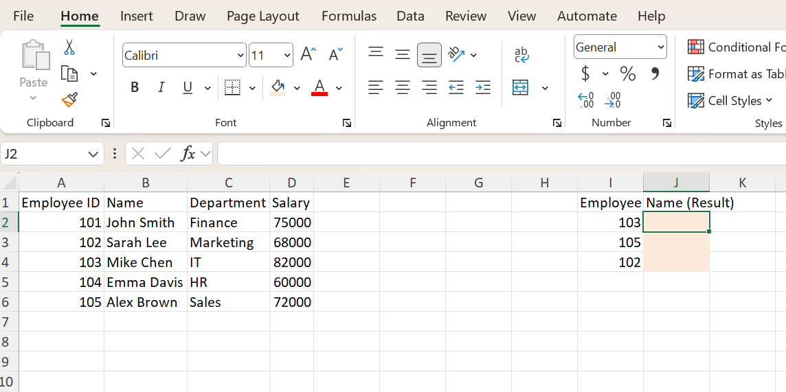
Step 1 — Click the cell where you want the result
Select cell J2 (next to the Employee ID input).
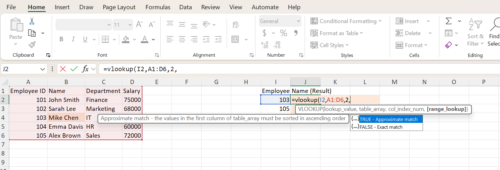
Step 2 — Type the formula
Enter:
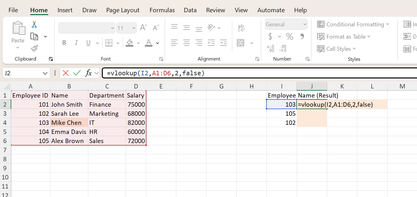
=VLOOKUP(I2, A1:D6, 2, FALSE)
The 2 tells Excel to return the value from the second column of the table_array (Name). The final argument is what trips most users up: always use FALSE for exact match. Omitting it — or passing TRUE — silently performs an approximate match and can return wildly wrong results on unsorted data.
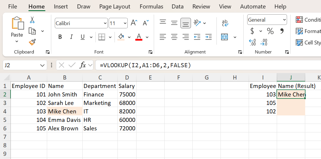
Step 3 — Press Enter
Excel returns Mike Chen — the name associated with Employee ID 103. Change I2 to any other ID and the result updates instantly.
Fixing VLOOKUP Errors
Most VLOOKUP errors fall into four common buckets. Knowing how to diagnose them quickly is what separates a working model from one that quietly breaks at 11pm the night before a deal.
#N/A— value not found. Either the lookup_value genuinely doesn't exist in the first column, or there's a hidden mismatch: trailing spaces or hidden/non-printing characters (note: VLOOKUP is not case-sensitive —"abc"and"ABC"match). UseTRIM()on the lookup column or the input value to strip whitespace.#REF!— wrong column index. Yourcol_index_numis larger than the number of columns in the table_array. Example: looking up column 5 in a range that's only 4 columns wide. Recount the columns or expand the range.- Wrong result — TRUE instead of FALSE. If you omit the last argument or set it to
TRUE, VLOOKUP performs an approximate match and returns the closest value less than or equal to your lookup_value when the first column is sorted ascending. On unsorted data, the result is effectively undefined. Always set the last argument toFALSEfor ID-style lookups. - Text vs number mismatch. The Employee ID
"103"(text, often imported from a CSV) does not match103(number). Check formatting on both sides — convert withVALUE()orTEXT()as needed.
Common VLOOKUP Mistakes
- Forgetting to lock the table_array. When you copy the formula down,
A1:D6shifts toA2:D7,A3:D8, etc. Use$A$1:$D$6to lock it in place. - Lookup value not in the first column. VLOOKUP only looks at the leftmost column of table_array. If your IDs are in column B and you select
A1:D6, it won't find them — start the range at B. - Hard-coded column index that breaks on column inserts. If someone inserts a new column in the middle of your table, your
col_index_numnow points at the wrong field. This is the number-one reason analysts switch to XLOOKUP. - Approximate match on unsorted data. Approximate match (TRUE) requires the first column to be sorted ascending. Otherwise the result is undefined.
VLOOKUP vs XLOOKUP
| Feature | VLOOKUP | XLOOKUP |
|---|---|---|
| Default match | Approximate (when omitted) | Exact (safe default) |
| Lookup direction | Left-to-right only | Any direction |
| Breaks if columns inserted | Yes (hard-coded index) | No (range reference) |
| Built-in if_not_found | No (wrap in IFERROR) | Yes (built-in argument) |
| Availability | All Excel versions | Microsoft 365, 2021, 2024 |
Pro Tips for Analysts
- Always pass FALSE explicitly. Don't omit the fourth argument — even if you mean exact match. Future-you (and your reviewers) will thank you.
- Lock your table_array with $.
$A$1:$D$6survives drag-fill;A1:D6does not. - Use named ranges for table_array in large models — easier to audit than raw cell references.
- Wrap with IFERROR for user-facing outputs:
=IFERROR(VLOOKUP(...), "Not found")keeps#N/Aout of presentation tabs. - Migrate to XLOOKUP for new builds when your team is on Microsoft 365 — fewer foot-guns, cleaner formulas, and no column-index drift.
When to Use VLOOKUP
VLOOKUP is still the right call when:
- You're working in a legacy model already built around it — consistency beats cleverness.
- You need to ship a file that opens in Excel 2019, 2016, or earlier, where XLOOKUP isn't available.
- You're doing a quick one-off lookup and the table is small and stable.
If you want a more flexible alternative — exact match by default, any-direction lookups, and built-in error handling — see our step-by-step XLOOKUP guide.
Frequently Asked Questions
Related Training
Ready to Get Faster?
Start practicing with hands-on Excel drills designed for financial professionals.