What is INDEX MATCH in Excel?

INDEX MATCH is a combination of the INDEX and MATCH functions used together to perform lookups. MATCH finds the position of a lookup value inside a column, and INDEX returns a value from the corresponding row of another column. Together they replace VLOOKUP and work in any direction.

Why is INDEX MATCH better than VLOOKUP?

INDEX MATCH works in any direction (including left), uses a direct range reference for the return column instead of a hard-coded column number, and doesn't break when columns are inserted or deleted. It's also typically faster on very large datasets and is often considered more reliable than VLOOKUP in financial models.

How do you use INDEX MATCH step by step?

Pick the cell where you want the result, then enter =INDEX(return_array, MATCH(lookup_value, lookup_array, 0)). For example: =INDEX(B2:B6, MATCH(I2, A2:A6, 0)) looks up the Employee ID in I2 inside A2:A6 and returns the matching Name from B2:B6. Always pass 0 as the third argument to MATCH for an exact match.

Why is my INDEX MATCH not working?

The most common causes are: (1) #N/A — the lookup value isn't found, often due to trailing spaces or a text-vs-number mismatch; (2) missing the 0 in MATCH, which switches it to approximate match and returns the wrong row; (3) mismatched ranges — INDEX return_array and MATCH lookup_array must have the same number of rows and start at the same row; (4) passing a 2-D range to MATCH instead of a single column.

INDEX MATCH in Excel: Step-by-Step Guide (Better Than VLOOKUP)

INDEX MATCH is the analyst's preferred lookup formula in Excel — more flexible than VLOOKUP, robust to inserted columns, and capable of looking up in any direction. This guide walks through the syntax, a worked example with screenshots, the most common errors, and why INDEX MATCH is often considered more reliable than VLOOKUP in financial models.

What is INDEX MATCH?

INDEX MATCH is a combination of two Excel functions used together to perform lookups. INDEX returns a value from a given range based on a row position, and MATCH returns the position of a lookup value inside a range. Combined, they replace VLOOKUP — and do it better.

Why analysts prefer INDEX MATCH:

It works in any direction — left, right, up, or down.
It uses a direct range reference for the return column, so it doesn't break when columns are inserted or deleted.
It can be faster than VLOOKUP on large datasets, especially in older versions of Excel.
INDEX MATCH is often considered more reliable than VLOOKUP in financial models — particularly in models that get edited, restructured, or audited frequently.

INDEX MATCH Syntax

The standard INDEX MATCH pattern is:

=INDEX(return_array, MATCH(lookup_value, lookup_array, 0))

return_array — the single column (or row) that contains the value you want returned.
lookup_value — the value you are searching for (e.g. an Employee ID in a cell).
lookup_array — the single column (or row) that contains the lookup_value. Must have the same number of rows as return_array and start at the same row.
0 — the match type. Always use 0 for exact match on IDs and codes. Omitting it defaults to approximate match and can return wrong results.

Step-by-Step INDEX MATCH Example

Here's an INDEX MATCH formula example in Excel. We'll look up an employee's Name by entering their Employee ID. The dataset has Employee IDs, Names, Departments, and Salaries in columns A–D (row 1 contains headers), with a small input panel where the user types an ID into I2 and the result returns in J2.

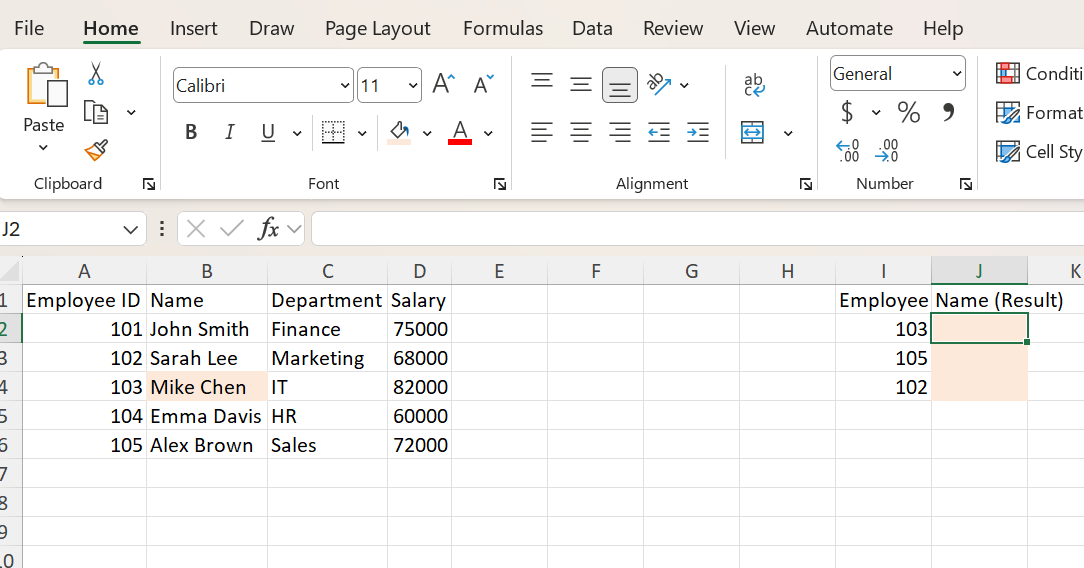
INDEX MATCH Excel example dataset with employee IDs, names, departments, and salaries in columns A through D — Sample dataset: Employee IDs in column A with Name, Department, and Salary in columns B–D.

Step 1 — Select the result cell

Click cell J2, where the looked-up Name will appear.

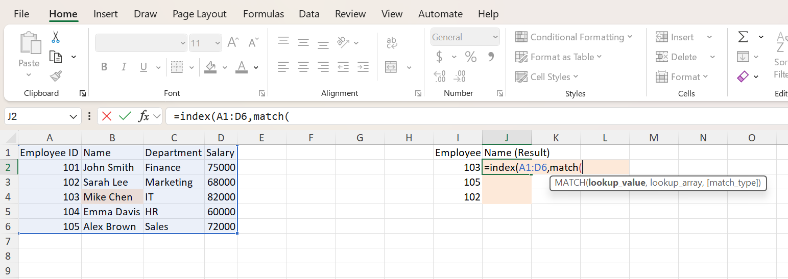
Step 2 — Start the formula

Begin typing:

=INDEX(A1:D6, MATCH(

A1:D6 is the full table. We'll use MATCH to find the correct row, then specify which column to return.

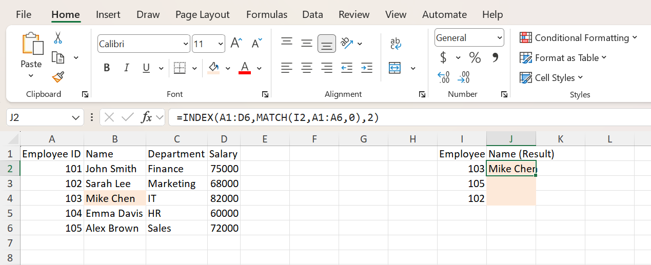
Building the INDEX MATCH formula in Excel with return array B2:B6 selected — Starting the INDEX MATCH formula with the return array (Name column) selected.

Step 3 — Complete the formula

Finish the formula:

=INDEX(A1:D6, MATCH(I2, A1:A6, 0), 2)

How it works:

MATCH(I2, A1:A6, 0) returns the position of the Employee ID in I2 within the lookup range (column A).
INDEX(A1:D6, ..., 2) returns a value from the 2nd column of the selected table (Name).
The final argument, 2, specifies which column of the table to return.
The trailing 0 ensures an exact match.

This version of INDEX MATCH uses the full table and explicitly specifies the column number to return — similar to how VLOOKUP uses a column index.

Note: this formula includes the header row for simplicity to match the screenshot. In practice, analysts typically exclude headers (e.g. A2:A6 and A2:D6) to avoid accidental matches on header text.

INDEX MATCH returning Mike Chen for Employee ID 103 in cell J2 — Result: Mike Chen returned in J2 for Employee ID 103.

Alternative INDEX MATCH Pattern (Analyst Version)

While the example above uses a full table with a column index, most analysts prefer a cleaner version that directly references the return column.

=INDEX(B2:B6, MATCH(I2, A2:A6, 0))

B2:B6 is the return column (Name).
A2:A6 is the lookup column (Employee ID).
MATCH finds the correct row.
INDEX returns the value from the specified column.

This version is more flexible and easier to audit, especially in financial models.

Both versions return the same result. The first approach mirrors VLOOKUP-style thinking (table + column number), while the second approach is more robust and preferred in financial modeling.

Why INDEX MATCH is Better Than VLOOKUP

Feature	VLOOKUP	INDEX MATCH
Lookup direction	Left-to-right only	Any direction
Return column reference	Hard-coded number (col_index_num)	Direct range reference
Breaks if columns inserted	Yes	No
Flexibility	Limited	High — works for any layout

For more on the older approach, see our step-by-step VLOOKUP guide.

Fixing INDEX MATCH Errors

Most INDEX MATCH errors fall into a few common buckets:

#N/A — value not found. The lookup_value isn't in the lookup_array, or there's a hidden mismatch — trailing spaces, hidden/non-printing characters, or a text-vs-number issue (e.g. "103" vs 103). Use TRIM() to strip whitespace, or VALUE() / TEXT() to align data types.
MATCH returning the wrong row. Almost always caused by omitting the trailing 0. Without it, MATCH defaults to approximate match and silently returns the closest value, which is rarely what you want for ID-style lookups.
Mismatched ranges. The INDEX return_array and the MATCH lookup_array must have the same number of rows and start at the same row. Otherwise the result will be offset (and may look correct on some rows and wrong on others).
Text vs number mismatch. IDs stored as text won't match numeric inputs (and vice versa). Convert one side with VALUE() or check the cell formatting.
Passing a 2-D range to MATCH. MATCH expects a single column or single row. Passing an entire table (e.g. A2:D6) returns #N/A or #VALUE!.

Pro Tips (Analyst Angle)

Always use MATCH(..., 0). Never omit the third argument for ID-style lookups — exact match should be your default.
Lock your ranges with $. $B$2:$B$6 and $A$2:$A$6 survive drag-fill; B2:B6 does not.
Default to INDEX MATCH for new financial models. Cleaner audits, fewer foot-guns, and resilient to column inserts.
Combine with SUMIFS or IFERROR for advanced patterns: =IFERROR(INDEX(B2:B6, MATCH(I2, A2:A6, 0)), "Not found").

When to Use INDEX MATCH

INDEX MATCH is the right call when:

You're building or maintaining a financial model that will be edited and audited.
Your dataset is large, and you care about calculation performance.
Your columns may shift over time (inserts, deletes, restructuring).
You need to look up to the left of the key column — VLOOKUP can't do this.
You're replacing legacy VLOOKUPs as part of a model cleanup.

Frequently Asked Questions

Related Training

Ready to Get Faster?

Start practicing with hands-on Excel drills designed for financial professionals.